Dense Camera Pose Estimation - Process & Lessons from the wild

The premise of all computer vision begins with images, and the foundation of all images are cameras. Cameras serve as the fundamental building blocks of all we do, the atom, in our lexicon, and ensuring their accuracy is crucial for addressing problems of deeper abstraction. Their influence is so encompassing and pervasive, that working on multi view geometry tasks with poor poses is a near doomed venture. At Avataar, faithfully projecting 2D image pixels into 3D space is imperative to our ambition of creating immersive 3D content. This projection is faithfully achieved by computing the camera ray for each pixel, and hence solving for accurate camera positions is the first step in the larger puzzle. 

Fig 1 - Left: Rendered image with rotation and translation error of ~ 10% , Right: Rendered Image with error of ~5%

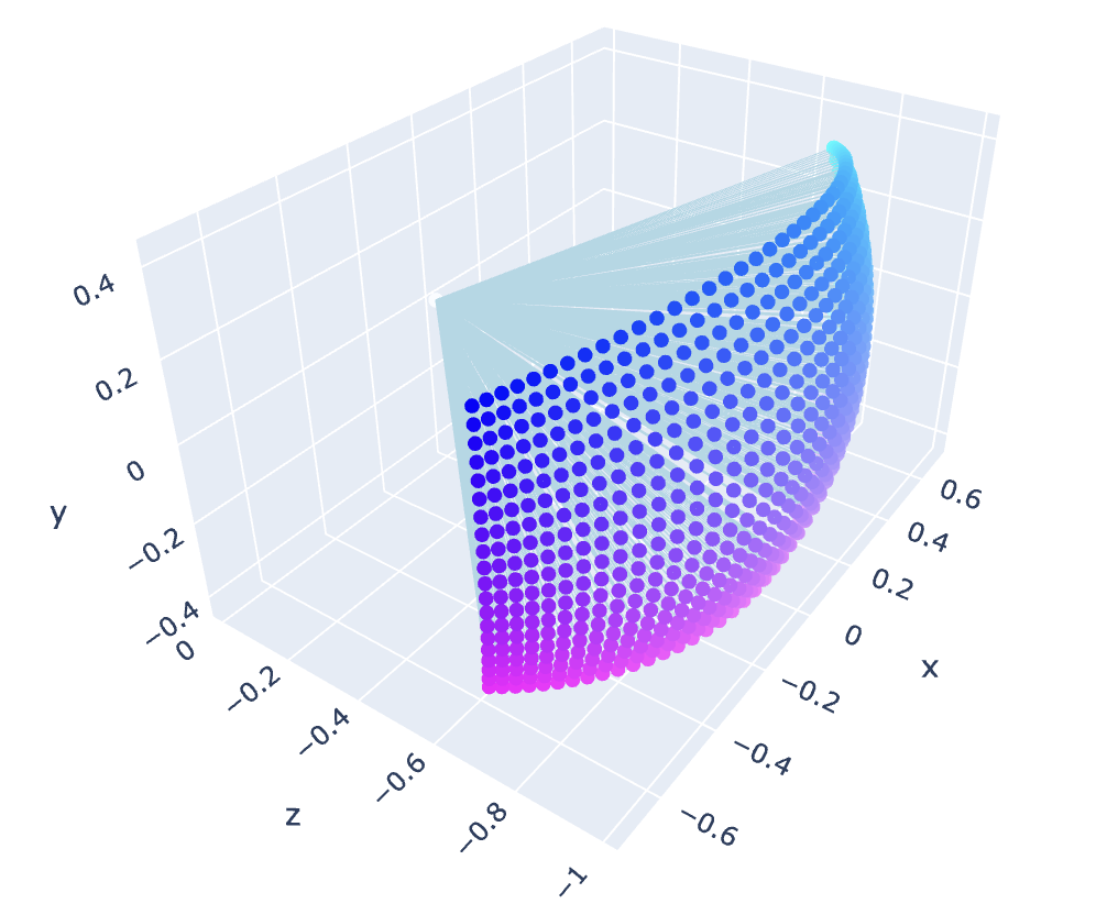
Our smartphone scanning application, Incarnate, which can be represented by a perspective projection camera model, harnesses ARkit - Apple's augmented reality development framework which in turn provides us with information regarding intrinsic and extrinsic properties of the camera being used. While information provided regarding the focal length of the camera, and its lens distortion can be accurately relied upon, its approximation of camera extrinsics, that is, its position and orientation remains riddled with noise, and hence we resort to a separate process of pose estimation in our pursuit of holistically accurate camera poses. 

Fig 2 - Perspective Projection model 

Most modern pose estimation problems are solved using SfM (Structure from Motion) or SLAM (Simultaneous Localization and Mapping) based methods. These methods generally provide 3D annotations by tracking cameras and reconstructing a dense 3D point cloud that captures the object's surface through the optimization of an objective function. While multiple off-the-shelf versions have achieved remarkable success in this task, we have found that a carefully crafted ensemble of various SfM implementations, along with some custom fine-tuning, works best for our object-centric use case. Outlining our steps and learnings below - 

Feature Extraction: Understanding the Nature of Images and Keypoint Detection

Our pose estimation pipeline, like most typical pose estimation pipelines, begins by understanding the nature of the images at hand. The first step in feature extraction aims to identify distinctive and salient points or regions in the images. These keypoints are crucial because they serve as anchor points that can be matched across multiple images, enabling the SfM system to establish correspondences between different views.Keypoints are typically detected based on their uniqueness and repeatability under varying conditions, such as changes in lighting, viewpoint, and scale. The quality of the resulting 3D model heavily depends on the method used for local feature extraction, making it of utmost importance. We have fine-tuned the Superpoint  feature extractor with our extensive repository of in house ground truth 3D data, to better understand features of primary importance to our use care. While passing full-sized 4032 × 3024px images through the VGG-style Superpoint encoder yields the most accurate point detections, it significantly increases computational complexity, leading to longer training times. We have found that downscaling to 1016×1502px and using a keypoint threshold of 0.005 provides us with reasonably good key points while maintaining speed.

Fig 3 - Key Points identified in the images

In the edge cases of textureless regions, keypoints are significantly scarcer and harder to detect, often leading to misleading results. In our image preprocessing pipeline, we try to identify these images and regions and apply contrast stretching, which involves applying the same contrast stretch to all images, or adding some point-patterns to alleviate the problem of lack of patterns in the image. 

Feature Matching: Keypoint Correspondences and Robust Matches

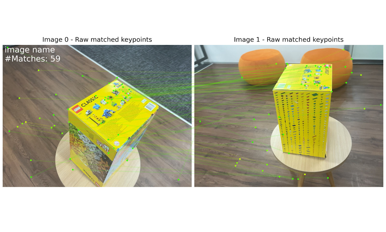
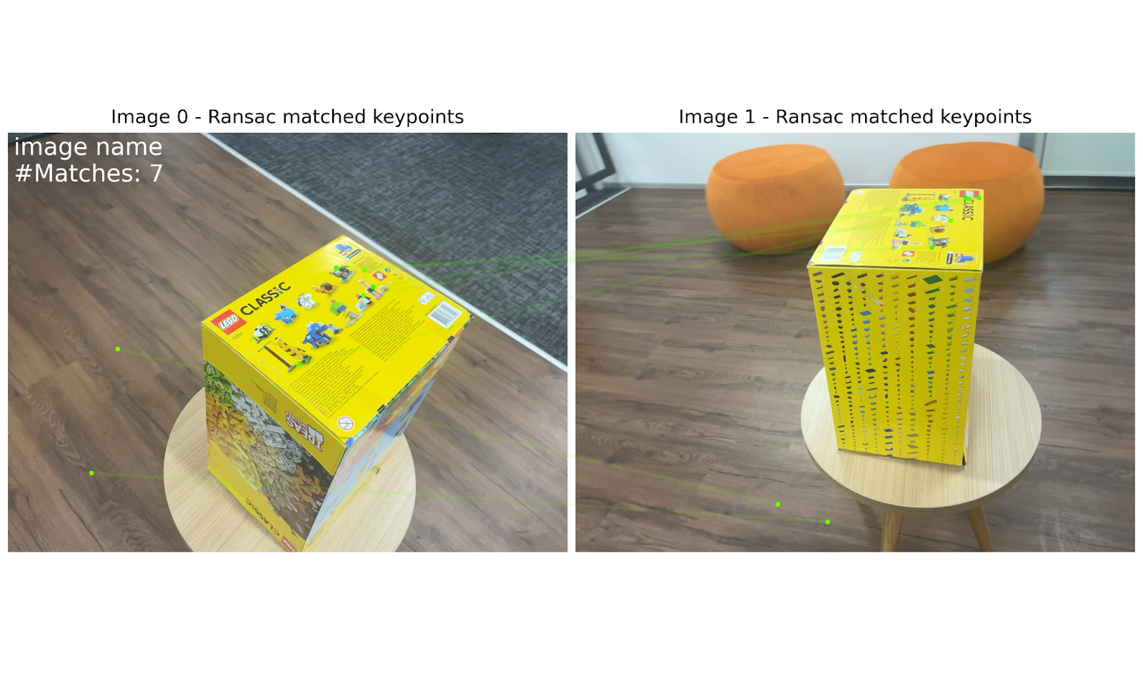
Once keypoints are identified, the next step is to match these key points between images. This involves finding keypoint correspondences that are likely to represent the same physical point in the scene. We use an ensemble of a graph neural network combined with a transformer based detector free matcher with a distance threshold of 0.7 to produce robust initial matches. We further filter the matches obtained using RANSAC for outlier removal to ensure that only correct matches are considered during subsequent stages of the SfM pipeline. Because exhaustive feature matching amongst all images is an expensive operation, we have found that matching each image to its top 20 most co-visible frames produces sufficiently robust feature matches.

Fig 4 - Initial Key Points Matches

Fig 5 - Filtered Key Points Matches

Triangulation: The Foundation of 3D Reconstruction

This process involves finding the intersection point of the projection rays from two or more cameras that correspond to the same feature in different images. The intersection point represents the 3D position of the feature in the real world, and serves as a solid initial pose estimate. This initial camera pose that best explains the observed 2D-3D correspondences is obtained via the PnP algorithm that calculates the position and orientation of the camera relative to the 3D points using non linear optimization techniques. 

Featuremetric Bundle Adjustment 

Once an initial pose is estimated via triangulation, we refine it via a feature metric bundle adjustment over the inlier correspondences. Bundle adjustment is the gold standard for refining structure and poses given initial estimates, and has stood the test of time. We use featuremetric bundle adjustment which along with reprojection error also optimizes a featuremetric error based on dense features predicted by the feature extractor neural network. In the bundle adjustment process we also take into account the uncertainty of initial detections and can recover observations arising from noisy key points that are matched correctly but discarded by geometric verification. 

Despite our best efforts to fine-tune and adapt our camera estimation algorithm for optimal performance in real-world settings, there still exist some edge cases relating to the object type, or surrounding environment conditions where the estimation algorithm spews an erroneous output. We have been able to classify these failures into distinct categories based on their causes.

Camera errors due to highly reflective objects

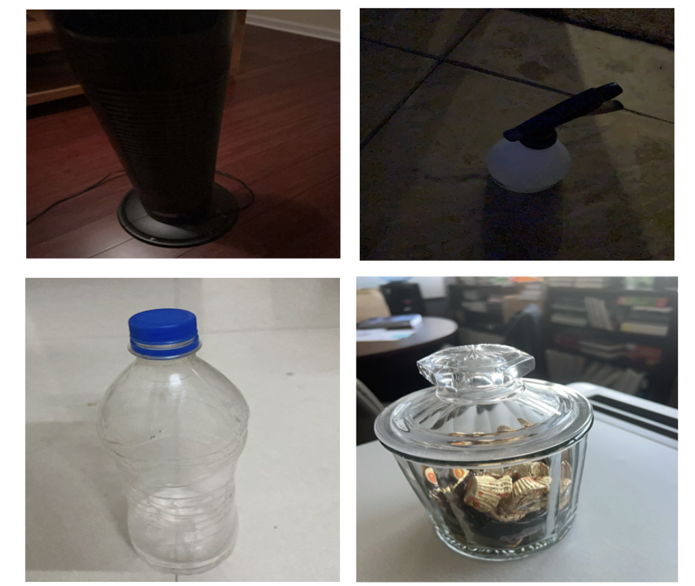
The first category of failures is related to camera errors caused by object material. Transparent objects, especially those with poor surrounding illumination, often lead to inaccurate camera estimation. Transparent materials bend light rays as they allow them to pass through, causing objects behind the material to appear distorted when viewed from different angles. This distortion introduces ambiguities in feature matching and depth estimation during the triangulation process. 

Fig 6 - Camera errors due to object material or environment lightning 

Camera errors due to capturer induced anomalies 

The second category of failures stems from anomalies introduced by the capturer in the scans. To paraphrase Tolstoy's famous lines in this context: 'All good captures are similar; each bad capture is unique in its own way.' Extending the analogy, there are multiple kinds of (preventable) failure modes of the camera estimation algorithm caused by aberrant capturer behavior, outlining the most common ones below - 

Scans which are done in very low-light environments, as seen in the first row of figure 7, are very susceptible to pose estimation failures. This is because there are significantly fewer detectable features due to the lack of contrast and low illumination, making it challenging for the algorithm to identify and track enough distinctive points leading to feature ambiguity. 

Another anomalous capture type are scans of objects done against a wall, as seen in the second row of figure 7. The Incarnate app provides circular trajectory camera rings and necessitates users to scan in this motion. While this isn't a necessity for the camera estimation algorithm per se, it will lead to incoherent bounding box placement and the user will have to resort to dubious camera angles to fulfill the Incarnate app’s circular trajectory conditions. This can necessarily result in incoherent camera estimation results.

As shown in the third row of figure 7, instances where the capturer inadvertently places their finger or body part in the frame or directs the camera's gaze to random objects in the surroundings for an extended period are also seen. These actions introduce new features, causing existing features to move unpredictably and be misrepresented, resulting in camera estimation failures.

Lastly, another commonly observed anomaly is when the object has a dynamic surrounding environment. As seen in the last row in Figure 7, dynamic elements, here, induced by external human movement within the frame cause inconsistencies in feature detection and matching, leading to significant uncertainties in the algorithm and erroneous pose estimations.

Fig 7 - Camera errors due to anomalies in capture conditions. 

Fig 8 - Camera Pose trajectories of failed pose estimations 

Over the years, we have collected thousands of such ‘good’ and ‘bad’ images and developed a camera confidence quantification algorithm that assesses image fidelity before reconstruction. Built with labels obtained with the assistance of manual annotators, and by assessing approximate distance of ARkit poses specific, our model filters out images that do not meet our quality standards both before and after the camera estimation step so that only the best images are used by the algorithms. This cautious approach ensures that pose estimation, and reconstruction failures, even in cases of scanning mishaps, are minimized.

Our next step in the pursuit of camera perfection is camera optimization which we incorporate during model training, more on which we will cover in an upcoming blog!